
Oil analysis and indeed all condition monitoring works on the principle of trending. If you don’t know what I mean by trending take a look at the graph below. It represents a series of samples including 3 tests over 9 samples, with sample 1 the oldest and sample 9 the most recent. So let’s ask a few questions of this data.

What’s a normal value for parameter 1 (the red line)?
Well you would be right if you said 20 and about 5 for green and 45 for blue. How do you know that? You know nothing about the sample type, machinery, frequency of sampling or tests performed but you got it right. Either some strange Jedi power mind reading trick is going on, or you just trended. You can pat yourselves on the back! For bonus points you might have noticed something happened at sample 4. To work out what, well let’s now make this a real sample from a methane gas engine.

This is the same graph but now with some names and context. The same rules apply but now we might think beyond sample 4 looks abnormal and into why. In this case landfill gas engines tend to have siloxanes in the gas and these make sand on combustion, which is abrasive. The lead and tin are wear to bearings as a result of this material, but thankfully it seems it was spotted quickly through trending and the issue was solved.
Why no weekly sample?
If anyone is into their gas engine oil analysis they will know gas engines are sampled weekly normally, especially landfill ones. So why was this customer only sampling monthly? Well, the gas quality in this case was fairly mild and the run hours on the engines were single digit hours a week and sometimes even a month at the time (this has since increased a bit). Ideally yes the customer would be sampling weekly, but the customer had decided to go monthly in this case. A few months after the events of this case study we convinced the customer to switch to fortnightly after a sample went from green to red in the space of a month when using our lab and we are reviewing falling in line with industry norms of weekly when the next budget is set for the sampling.
So why was there no November sample?
Well the engine failed in October, just 2 days after the October oil sample. Strange thing though, the report came back the day after the failure with a green tick on it. So clearly something was up. It could have been a sudden unpredictable failure with a proverbial spanner in the works, but perhaps it was detectable. So how? Well the answer is to do with normal and abnormal wear. To explain this. Let’s rewind and explain what is normal wear.
Can wear be normal?
Yes everything wears to some extent. This is normal. Traditionally these are small particles and as things go wrong they go bigger and sometimes up to large visible size particles. 15 microns is internationally recognised as the cut off between normal and abnormal wear particle sizes. Now you will get a little wriggle room around this but the majority of the particles in normal wear will be smaller than 15 and the majority will be above 15 sometimes in the 100s of microns when abnormally sized.
Is size the same as number?
Your reports and lab reports give a number in ppm or mg/kg of how much wear is present. However they give no details of size. It may surprise you to find out that ordinary oil analysis does not detect every size of particle. In fact it detects only accurately particles less than 5 microns although some may argue up to 8 microns depending on instrument designs. For those observant amongst you you may be thinking, hang on, that is only about ⅓ to ½ the normal wear? What about the abnormal stuff? Well that’s a good point. This is a known issue with oil analysis wear metal detection. That is why people use trending and a normal distribution of wear.
To explain this let’s imagine we have this distribution of wear below in a sample. Now it’s only the yellow bit we can actually measure with oil analysis, but we can extrapolate based on that amount of yellow what the real wear may be and base trends and limits on that bit of yellow assuming a normal distribution of wear particle sizes.

That’s great, but what happens if you have something really abnormal going on, so the “skew” goes well into the abnormal size of particles. Well this is where the issue occurs. Let’s go back to our monthly sample example above. We have 18ppm of lead wear in June in our example. That’s great, it’s back around the normal level and moreover is actually a little lower than before. Job done surely? Well, remember at this point we can only detect particles less than 5 microns (the yellow of our graph). What would happen if the wear took a skew towards larger particles and became an abnormal wear mode. If you take a look at the scenario below the skew has moved towards an abnormal distribution. We are still only measuring the 5 micron particles though aren’t we? So that means there is a whole lot of wear not being picked up that is pointing to a serious issue.

So what’s happening?
Well following the May sample the customer did an oil change. All good and the contamination was removed. The gas seemed stable. However, in this case, the contamination was not from the gas and it was something I first noticed when I was shown this data. Why you might ask? Well if the wear was from siloxanes in the gas I would expect to see a whole load of piston, ring and liner wear from the combustion chamber area where it’s being generated. However these looked all low with no Alumium, chromium or iron wear the classic elements for upper cylinder wear.
At this point, If you are confused as a general recap here is a guide to engine metallurgy to keep you up to speed as I discuss this.

So to recap, if dirt, sand or something abrasive is entering the upper cylinder in the gas flow why are the piston, rings and liner completely un-affected? How is the silicon magically getting to the bearing to cause tin and lead wear? Well the answer is simple, it’s not coming from the gas. There is another route of entry…and that’s the oil.
The oil with the smoking gun?
If the oil is contaminated this can put oil directly into the sump and close to the crankshaft bearing feed of lube oil. What happened was not a gas spike, but a dirty oil top up causing wear to the engine. The lab they used to their credit picked this up, and the customer trying to fix the problem drained the oil and refilled it with the same oil they had been topping up with, what neither party knew was the bulk storage tank the oil was being filled into on site was in very poor condition and was very dirty. The oil change rather than removing the contamination actually filled it with a whole load more contaminants. You may notice the slight increase in silicon in July too, but the customer too had also added some new gas scrubbers to the engine feed to try improve the gas which and the silicon now was not mostly siloxane and some sand, but was now entirely dirt/sand from the sump. The wear looked normal so all was good. The problem was this was only the tip of the wear iceberg.


The wear under the water line got bigger and bigger and because it got heavier it pulled the iceberg down making the wear look even smaller above the water. This eventually led to a failure. So how did I get involved in this scenario? Was it my lab doing the testing? The answer is no, and I first heard of this company only after they contacted me to ask could I analyse an oil filter and help them identify the cause of a bearing failure.
What did the analysis find?
Well we found cutting wear in the system. Quite a bit of it to be honest. Here are a few microscope images from the oil pulled from the failed engine sump. Particles ranged typically from approx 35 microns up to 2000 microns (2mm) in places. The customer also commented there were visible fine grooves in one of the non failed bearing shells too.

I said let’s have a check of the lube oil storage conditions. The customer had 2 large tanks on site. One tank was about 3 years old and looked fairly good condition whereas the other was approx 15 years old and had a crack on the cover of the site glass, standing water on top of the tank as it had a flat top, whereas the newer design had a slightly rounded top to allow water run off. The oil pump used to connect to either of the tanks and pump in oil from the tank to the engine looked the worst though covered in what I thought looked like pebble dash.
I suggested we do a particle count on the new oil in the tank (there is not much point doing this on used engine oils), but useful on the new oil and after running off 20 litres from each tank we had an iso code of 21/19/14 in the newer tank and 24/22/18 in the older tank. Remember this is after running off some oil from the bottom of the tank. For reference a typical new engine oil would be around 20/18/15 and each time a code goes up it gets twice as dirty. So the oil in the newer tank was a little dirtier on the smaller >4 and >6 micron scale and a little cleaner on the >14 micron than new oil. Whereas the second tank 16x, 16x and 8x dirtier than new oil.
Should you do particle counts on engine oil’s routinely?
In short No. You end up measuring oxidation products, carbon based deposits and the use of the data becomes less useful. In reality I only used this on the new oil to check the cleanliness of the new, not used engine oils. On used engine oils particle counting is an estimate at best and is very poorly reproducible to make anything meaningful to the client. In gas engines Silicon is a far better indicator for checking for silica based contaminants in oil. Hence, for those considering using particle count on engine samples, i would rule out laser counts immediately and possibly as part of a research project you may wish to do a microscopic count, but for routine analysis this is not needed. For those wondering would ISO code have detected a problem on the used oil samples there was a 1 code increase coinciding with the increase in silicon, but there was a 2.5 code variation on the months leading up to this sample showing the accuracy of sampling engine oils for particle counts was actually worse than the difference seen when the problem took place.
So now we identified the issue the customer could actually get their housekeeping in order and clean up the problem tank.
The customer was thankful for the help and I suggested why not try our lab (forever having my salesman hat on). However, the customer used a couple of words I can’t use on a blog post, but suffice to say he thought it was a waste of time as it didn’t pickup the issue. I suggested that our acid digestion technique LubeWear would have helped them as it breaks down larger wear particles to smaller ones that can be detected. I was expecting to get a trial on another engine side by side but little did I know I was able to get one on the failed engine. How you might ask?
Time travel
I often do side-by-side trials with customers and have to often disagree with their current labs findings when we say there is or isn’t a problem based on our LubeWear analysis. As mentioned, I explained to the client about how LubeWear could potentially have helped identify the problem before the failure and we should sample other engines to see if there were similar problems. I was expecting at this point the customer to order some bottles and test their oil over the next few months. However, I was told “no need” and the customer had the samples from the engine. Confused as surely the lab would have disposed of the samples by now if they asked for them to be returned, I found out the customer used to work in marine insurance for large 100 million dollar vessels and always when they took samples retained an “on board” sample too for 12 months in case they needed second opinions. When the customer left the Navy and got a land based job he followed the same practice. I was taken to a small steel portacabin and the gentleman opened one of the cupboards and there was over 100 samples he had retained from various engines, each in an ordered row by engine number and colour coded. I thought he could come organise my kitchen next. For those of you wondering that’s a lot of lab analysis costs, the customer had purchased a load of empty bottles not including testing too for this purpose. Anyway, this I knew was the holy grail of case studies, as when do you ever get all the historical samples after a failure to prove the value of your own service? The customer gave me the samples to test and for ease let’s just focus on the lead for this article. The lead by the original lab is in green (note a different scale now as we have some higher numbers than before). Now over Feb to May (the january sample was lost at the old lab so we actually got one they didn’t measure too) the results were fairly similar on the engine, but after May they started to really differentiate. At first, only slightly up to about July and then they really rocket apart; why then? Well, the engine hours went up a lot in July as it was not run much between May and July but towards the end of the summer hours went up, not massively as the oil would have been changed a few times if run continuously in that time, but enough to get some decent lead wear it seems.
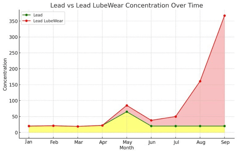
So when would LubeWear identify issue.
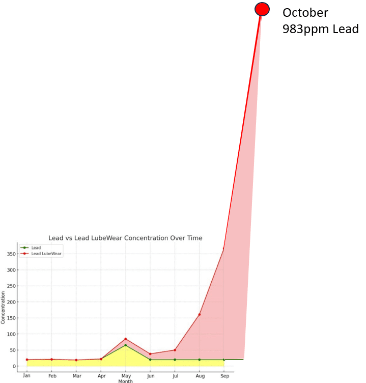
Well the difference was seen in May in both standard and ICP, but the wear never truly returns to mainly small particles at this point. In June, even though there was some differentiation in the wear, the direction of travel by trending was coming down for both, so I would be inclined to say things were getting better. Up until June we all agree. However in July and August things really start to get bad and so much so I would have likely called the client in this circumstance to ask what was going on with the engine. You notice my graph finished in September. There is a reason for that and its to do with space. Well, space on the page, as if I showed the full graph you would likely guess something had happened. Remember the red shaded area is abnormal wear. It doesn’t take a lot of skill to see something is amiss. Here is the graph including October.
Trending still needed?
You may be thinking I still need trending to identify the rise like in this instance. But, the fact is I don’t. If i take any snapshot sample at any point in that list I can tell if something is normal or abnormal just by looking at the small-to-large particle ratio. In most cases, that’s generally all I get, as normally the customer has already taken action based on our report before you see such beautiful case studies as this showing the benefits of LubeWear. However, lets take some snapshot samples, no history of standard ICP vs LubeWear.
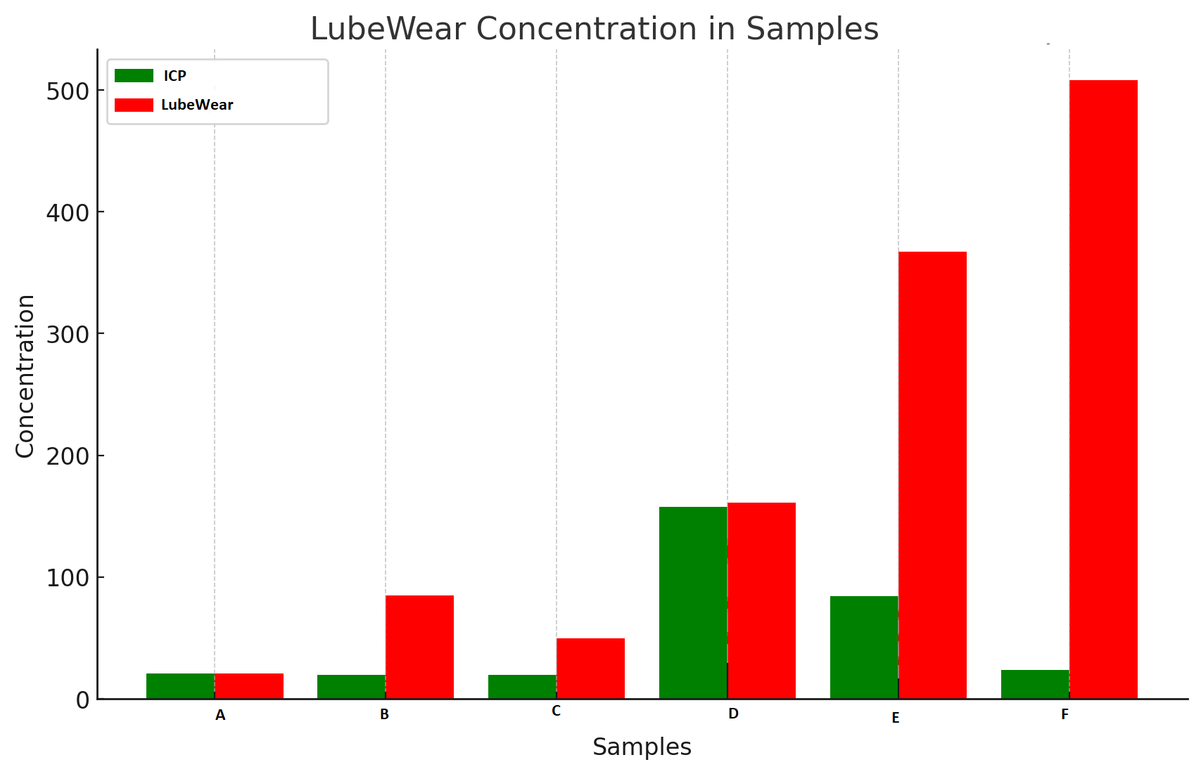
In sample A everything looks normal, B not too good as there is a skew towards larger particles, C the same. D is a strange one, as there is a lot of wear but all small. In this circumstance the wear is related to length of time in use rather than something bad going on, so an oil change would likely solve this. E and F are clearly in poor states, and F more so because of the skew. See…..no trending needed for these examples. Trending helps, but is not essential with LubeWear analysis and often we can help you before you get to the point that the trend is required to highlight an issue.
Overall, it is very rare you get to basically go back in time and reanalyse the samples leading up to a failure, and this is one of the most enjoyable case studies I have had to write up and is a perfect example of how LubeWear analysis can identify serious wear issues much earlier than traditional trending techniques and also of the dangers of relying purely on those small less than 5 micron size particles to make a decision.
If you want to discover the newer way to diagnose your lab analysis data using LubeWear get in touch using the contact us button below.